Excel: Formatting and Formulas

Are you not that familiar with Excel yet? Then it is advisable to first read the article ‘Excel: starting with the basics’. It tells you how to enter data into Excel cells and how to change the format.

To show in a practical way how to easily format cells and perform simple calculations, let’s make a small table. You can also create such a table for a variety of subjects, such as your monthly fixed costs. Type in cell A1 Fixed charges.

Leave a cell below it blank and type in A3, A4 and so on Rent, Gas/electricity, Water, Groceries. At the very bottom, tap “Total.” In cells B2, C2, and further to the right, type the months of the year. If necessary, make the columns a bit wider to see the words well.

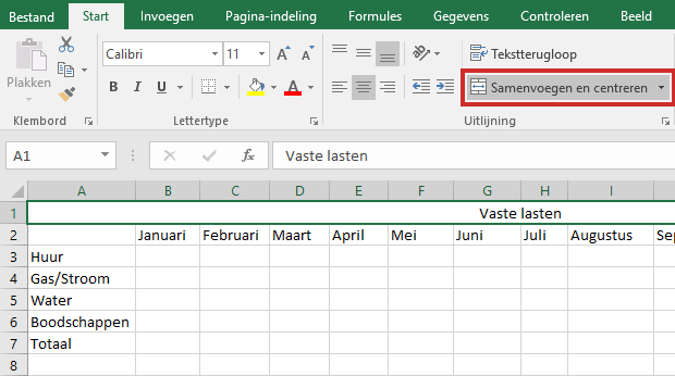
The table is already starting to look like something. It would be nice if the cell with ‘Fixed charges’ could be placed in the entire width of the table. This can be done by merging cells.

• To do this, select cells A1 to M1. Click in cell A1 > press the Shift-button > click in cell M1.
• The ‘Home’ tab contains the ‘Alignment’ group.
• click on Merge and Center.
  
• The cells become one with the text in the middle (see image above)
• If you just want to merge cells without centering, click the triangle to the right of this option. click on Merge cells.

With different colors the table is a bit clearer. Here’s how to give cells a nice color:

• Select cell A1.
• In the ‘Start at’ tab, click the ‘Cells’ group layout.
• Click on in the drop-down menu at the bottom Format cells.
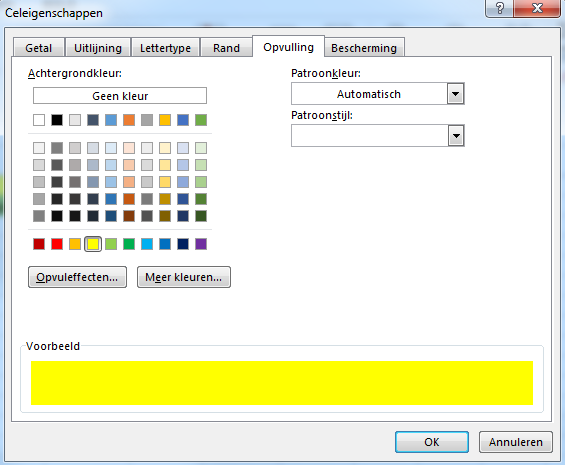
• The window called ‘Cell Properties’ or ‘Format Cells’ will appear.
• Then select the ‘Fill’ tab.
• Choose a fill color, for example yellow. The Preview box shows the color.
• click on OK. The cell is now yellow.

We make the left side green in the same way, just like the months. We make the row with the future total amounts orange. In this way a nice table is slowly created.

In the step above you opened the ‘Cell properties’ window. There you will not only find the ‘Fill’ tab for colored cells, but many more options. For example, take a look at the ‘Border’ tab to provide one or more cells with a visible border. Or choose a different letter on the ‘Font’ sheet. The possibilities to design cells to your own liking are very large!

Now let’s calculate. In the table we enter the amounts of our fixed expenses for the month of January, in this example 500, 100, 50, 250. Excel can add these amounts for you. In this example that is not such a difficult calculation, but if you understand the principle, you can also perform more complicated calculations.

Select cell B7, which should contain the result of the sum. Above the cells is an empty white bar with ‘Fx’ to its left. That’s the formula bar, where you can select formulas for calculations.

• click on fx. The ‘Insert Function’ window appears.
• In the panel, click Sum. That’s the formula for simple calculations.
• Then click on OK.

A new window will appear. It says ‘B3:B6’. That does not mean ‘B3 divided by B6’, but ‘the sum of B3 to B6’. That’s exactly the sum we want to know! click on OK. Cell B7 now contains the answer to the calculation.

You can also create other types of sums. We discuss formulas in more detail in the article ‘Calculating with Excel’.