Smart tricks for Excel

When you let Excel perform calculations, sometimes the result does not fit in a cell. You will then see ‘######’ instead of a number. Then adjust the width of the cell as follows:

• Move the mouse pointer to the appropriate column until you reach the letters.
• Move to the right until you reach the column divider.
• The mouse pointer changes to a black cross with horizontal arrows . Now double click on the column separator.

Excel adjusts the width so that the number fits exactly.

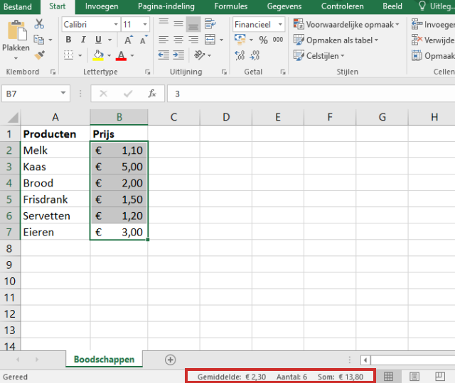
You have a series of numbers in Excel. Now you want to add some of those numbers (or the whole series) together and quickly see the result. Excel has an option for that in the status bar. Bet you hadn’t noticed yet? But try the following:

• Select a few numbers in Excel.
• Look at the bottom right of the status bar.

You will see the average, the number of selected numbers and the result of the sum.

Remark: right-click anywhere on the status bar. A menu will now open with which you can display ‘Minimum’, ‘Maximum’ and ‘Numerical count’ in addition to ‘Average’, ‘Number’ and ‘Sum’. Click on an entry to set it up. The difference between ‘Numeric count’ and ‘Count’ is that the latter counts all selected cells, while the former only counts the cells with a number value.

Sometimes a text is too long. No need to let that text run across the entire width: divide it over several lines in one cell. That’s easy. Type the text and press the keyboard shortcut Alt+Enter if you want to break it (always), then just continue typing. At the end of the text, press the Enter key. The cell does not become wider, but only higher, so that the text is visible in its entirety.

If you’re creating a table of titles, you’ll want to keep seeing it as you scroll down. So secure them!

• In the Ribbon, click on the tab Image.
• click on To block and select the appropriate option.

You can choose from:

1. Block titles
2. Block top row
3. Block first column

Option 2 and 3 are the most useful: with 2 the top row remains visible and with 3 the first column.

Use the F4 function key to repeat the last operation. That can save a lot of time. Suppose you change the text color of one cell. Click on the next cell and then press F4. Now the text color of this cell has also been adjusted. You can also select a range of cells and use F4 to make them change color all at once.

If you know someone’s date of birth, you can have Excel display their current age.

• Type the date of birth (for example, 11/13/1955) in cell A1.
• Select the following formula: =ROUNDDOWN((TODAY()-A1)/ 365.25;0)
• Copy the formula with the keyboard shortcut Ctrl+C
• Paste the formula with the keyboard shortcut Ctrl+V into the cell where you want to see the age.
• Press the Enter key.

Note: the formula contains the reference to cell A1, where the date of birth can be found. If you have the date of birth in another cell, replace ‘A1’ with the cell where you entered the date of birth.

A large Excel file can easily contain duplicate data. Removing those duplicate values ​​is a simple job:

• Select the column that is believed to contain duplicate values.
• Click on the tab Facts.
• In the Data Tools group, click Remove duplicate values or on Remove Duplicates.
• click on OK.
• It says how many duplicate values ​​have been removed. click on OK.