Workshop Getting started with Excel (part 2)

Niels Brouwer

Excel, from the Microsoft Office stable, is perhaps the best-known program for creating spreadsheets. Making budgets, drawing up graphs, filtering in collections, it’s all possible in it.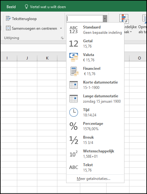
In PC-Active 322 you learned how to create a new worksheet, what a cell is and which tabs there are in the ribbon. Here we take it a step further and really start using the program.

NUMBER NOTES
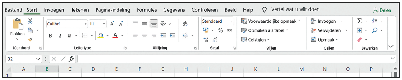
What kind of numbers do you want to work with on your spreadsheet: numbers, currency, percentages? You set this in Number, which can be found in the Home tab, in the middle of the ribbon. (The names of the various tabs are always at the bottom of the ribbon.)
When you enter a number in a cell, let’s say 50,000, you can specify what shape this number should take. You can choose from, for example, currency, percentage, a fraction, etc. If you want to have a number in a cell as the amount in euros, take the following steps: type the number in the cell and make sure that the format is not Standard stands, but on Financial† Click on the arrow next to Standardso that the menu rolls out and choose the option Financial† There is also a hotkey available, you can read about that later. To display all the numbers in a particular column as amounts, select that entire column by clicking the letter at the top of the horizontal line, then click Financial in the ribbon.

PERCENTAGE
In addition to financial notation, you can also display numbers as percentages. You do this by following the same steps as above, only instead of Financial click, now select Percentage† Below the menu bar you will see five keys. Click the percentage icon. You immediately see the effect. For example, if the selected cell contains the number 0.25, this will be 25 percent. If the number is 1 in the cell, the percentage will be 100. So the decimal point moves two places to the right of the number.

THOUSAND NOTATION
When you use large numbers, it can be useful to separate the thousands with a period. Enter the number in a cell. Then click on the shortcut key 000, to the right of the percentage icon. You will see that the amount will be adjusted immediately.

When you click, you will see that an extra digit is added after your entered number

NUMBERS AFTER THE COMMA
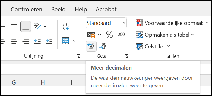
For example, if you write 10.50 in a cell, Excel automatically changes it to 10.5. The program assumes for a calculation that the zero is superfluous. If you want to have that zero in the picture and always see two or more digits after the decimal point, this is of course possible. To do this, click on the relevant cell(s) or column and go back to the ribbon where you see the five icons in the tab Number† Click the left arrow icon followed by 0.00† This stands for More decimalsyou see this when you rest your mouse on this key.
If you see an unnecessary number of digits after the decimal point in your cell, you can easily change this with the icon for Fewer decimals, by clicking on the appropriate icon. You will see that the number is rounded off after the decimal point, but if you double click on the cell, you will see the real value. Suppose you enter the number 17.89 and you click on More decimals, you will see that the number changes to 17.9. If you double click on the cell, you will see the real value again, namely 17.89.

Open the Cell properties for more options to shape the number

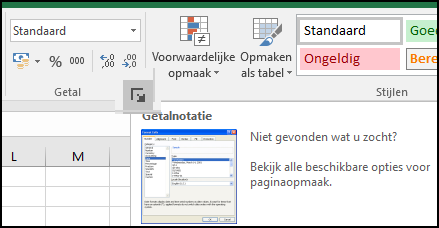
CELL PROPERTIES
In addition to the five icons in the Number tab and the keyboard shortcuts in the ribbon, you have even more choices for numbers, namely in the window Cell properties† You open this by clicking on the diagonal arrow at the bottom right of the Number tab. A window will now open with all cell properties. You have quite a few options here, in this case we take the cell property Number as an example. You can indicate several preferences here. When you are busy entering numbers in Excel, such as 12.50, Excel immediately changes this to 12.5 when the choice in the tab Number on Standard state. As mentioned, it sees the 0 as redundant. You can indicate how many decimal places you want in the worksheet. You can also indicate whether you Separator want to apply. This means that there is a period after the thousands. You also have the choice whether you Negative numbers in the color red or black, with or without a minus sign.
There are many other properties, also known as notations. With the notation Currencies can you under Symbol choose various currency symbols. Here you can also indicate whether you want to display negative numbers in black or red.

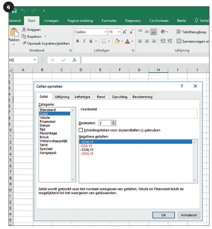For example, under ‘Currency’ you can indicate in the cell properties that you want to display a negative amount in red

Also you have the previously discussed notation Financial† This one is similar to Currency, the difference is that at Currencies the currency sign is right next to the amount and at Financial on the left side of the cell. Further gives Financial no zero values ​​again as a dash and finally you don’t have the choice to display negative numbers in red. With the notation Date set what a date should look like. when you’re on Date clicked, you will see on the right side of the window Type where you can indicate how you want the date displayed. At the notation Time the same applies to displaying times: the examples below Type show how a time can be displayed. With the notation Percentage display a number in percentage.
Of fracture display your numbers as fractions. For example, you see the number 1.125 as 1 1/8. Note that if you want to enter a fraction directly into a cell as a fraction, you must first enter the whole number, then a space and then the fraction. If you only enter 1/9, Excel displays that as the date September 1. Enter the whole number first, such as 0, followed by a space, and then the fraction. If you have already set the cell in advance, you do not have to enter the whole number.
Furthermore, there is the property Scientific† In the scientific way of writing, or so-called exponential notation, 12,500 looks like 1.25E+04. This stands for 1.25 times 10 to the fourth power. Do you choose the notation Text, then Excel displays the numbers as text at the left edge of the cell, just like regular text. Excel can just calculate with it.
The notation Special is for telephone numbers, among other things. When you enter a phone number with the 0 in front, this zero disappears in the Standard-display. With the notation Special and the option phone number this is not so. With the option Place there is a dash after the third digit, as with large cities and with the option Regional the dash comes after the fourth digit. Do you do this in Belgium and see below Type these options do not, then change in this window under Location the option Dutch (Belgium) in Dutch (default)† When you finally get the notation Amended click, you can enter a format code.

MAKING CALCULATIONS
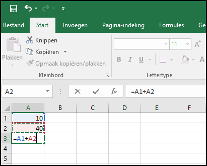
You can easily make calculations in the formula bar in the worksheet, which we discussed in part 1. The formula bar is the long white bar located directly above the worksheet. In this case we click on cell A1. We are going to fill in the sum 12+4. we fill in: =12+4 and click on Enter† In cell A1 you immediately see that the number 16 is there. It is important that you always start a calculation with a ‘=’ and end with Enter† Then we select cell A2 and in the formula bar we write =1+3. You will then see that there is automatically four. What you can do next is add cells A1 and A2 together. In that case, type =A1+A2 in the formula bar. You can make formulas in as many cells as you want and add, multiply or divide as many cells as you want. To subtract, enter a ‘-‘ instead of a ‘+’ in the formula bar. For multiplication, the sign is an asterisk

Excel part 2.6 calculation with cell reference 2
MAKING CALCULATIONS WITH CELL REFERENCES You can also reference formulas in another cell. To do this, enter the number 10 in a cell, for example A1,. If you then select cell B1 and enter ‘=A1’ in the formula bar and click Enter click, you will see that the same number as A1 is entered in B1. You can also calculate with cell references. Cell A1 contains the number 10. Enter, for example, cell A2 the number 40. Then you first enter a ‘=’ in the cell below, A3. You then click on cell A1. Then fill in the plus sign in A3 and click on A2. When you get up afterwards Enter

click, you will see that the number 100 will be placed in cell A3. SEND SEQUENCE

auto sum 2

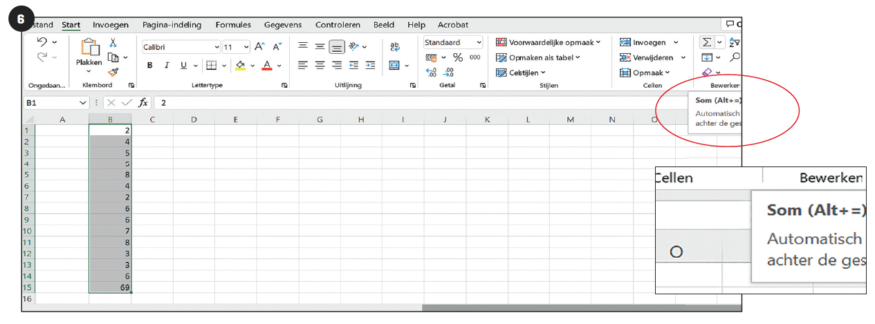
‘Autosum’ is a quick way to make simple calculations
AUTOSUM We don’t want to withhold one last trick from you: the handyAutoSum † With this you can easily add cells together. All you have to do is select the cells you want to have added up. In this example, we entered random numbers from cells B1 through B14. You select these cells by dragging the mouse. You can also click on B1 and then theshift Press key while clicking on the last cell (B14). Then click on the top right of the ribbon AutoSum in the tabTo process

† You will see that in the cell below the selected cells (in this case in B15) a number will immediately be placed: the result of this addition. The AutoSum can do a lot more, but we have to leave it at that in this Excel introduction.